EdgeAttend: Distributed Real-Time Attentiveness Detection on the Edge

Team: Veera Subrahmanya Vignesh Vemula, Tata Umesh, Botta Lokesh Appa Rao, Anumala Sadhan.
Code: GitHub Repository
1. Problem Statement, Motivation & Objectives
Problem Statement
Remote work environments have expanded rapidly, yet existing meeting room monitoring systems struggle to meet real-world requirements. Traditional cloud-based solutions introduce significant latency (200–500 ms) and rely heavily on stable internet connectivity, limiting their reliability in dynamic or bandwidth-constrained settings. Meanwhile, on-device approaches either depend on costly specialized hardware such as GPUs to run computationally intensive models or compromise accuracy to achieve real-time performance. This highlights a critical gap in developing a solution that can deliver low-latency, reliable and accurate monitoring without reliance on high-end hardware.
Motivation
This project addresses the growing need for real-time attentiveness detection in distributed meeting environments. As remote work becomes the norm, maintaining participant engagement without compromising system reliability has emerged as a key challenge. Existing solutions often rely on cloud-based processing, raising concerns around latency and network dependency. There is a strong need for systems that can operate efficiently on everyday devices while ensuring minimal latency. Enabling such capabilities can significantly enhance remote collaboration by providing seamless, responsive and trustworthy engagement monitoring without requiring specialized hardware or constant connectivity.
Objectives
- Develop a real-time edge AI system that detects participant attentiveness locally on client devices with low end-to-end latency.
- Achieve high accuracy on binary attentiveness classification (attentive vs. non-attentive) while maintaining better recall.
- Compress the model using INT8 quantization and explore pruning trade-offs to ensure deployment on standard CPUs without GPU requirements.
- Design a multi-threaded server-client architecture supporting 5+ concurrent clients with centralized grid visualization, enabling distributed meeting room monitoring without cloud backend.
- Implement Edge Computing, ensuring all inference occurs locally on client devices, server aggregates attentiveness label.
2. Proposed Solution
High-Level System Architecture
The proposed solution implements a distributed edge AI system for real-time attentiveness detection in meeting environments. Unlike cloud-based alternatives, inference executes entirely on client devices using a lightweight MobileNetV2 model compressed via quantization and pruning techniques.
-
Client-Side Edge Inference: Each participant’s device runs local attentiveness detection on their webcam feed, producing mood labels (Attentive/Not Attentive)
-
Server-Side Aggregation: A central server receives mood data from all clients, assembles a real-time grid of annotated video tiles, and broadcasts updates back to all participants.
Overall Pipeline: Data → Model → Deployment → Output
┌─────────────────────────────────────────────────────────────────────────────┐
│                         DATA COLLECTION & PREPARATION                       │
├─────────────────────────────────────────────────────────────────────────────┤
│  • DAiSEE public dataset: Binary labelling of engagement scores             │
│  • Preprocessing: Face detection → 160×160 crop → augmentation              │
│  • Train/val/test split: 70%/15%/15% of 10,000 images                       │
└─────────────────────────────────────────────────────────────────────────────┘
                                     ↓
┌─────────────────────────────────────────────────────────────────────────────┐
│                    MODEL TRAINING & OPTIMIZATION                            │
├─────────────────────────────────────────────────────────────────────────────┤
│  • Architecture: MobileNetV2 backbone + lightweight custom head             │
│  • Training: 2-stage strategy (head-only 10 epochs, fine-tune 10 epochs)    │
│  • Compression: INT8 quantization, Structured and unstructured pruning      │
└─────────────────────────────────────────────────────────────────────────────┘
                                     ↓
┌─────────────────────────────────────────────────────────────────────────────┐
│                    DEPLOYMENT ON EDGE DEVICES                               │
├─────────────────────────────────────────────────────────────────────────────┤
│  • Runtime: Python + PyTorch (CPU) + OpenCV on client machine               │
│  • Inference: Local batch processing (5 frames) for smoothing               │
│  • Communication: TCP messages (frames, mood labels) to server              │
│  • No GPU required, runs on standard consumer hardware                      │
└─────────────────────────────────────────────────────────────────────────────┘
                                     ↓
┌─────────────────────────────────────────────────────────────────────────────┐
│                    SERVER AGGREGATION & VISUALIZATION                       │
├─────────────────────────────────────────────────────────────────────────────┤
│  • Multi-threaded TCP server : handles 8+ concurrent clients                │
│  • Dual grid output:                                                        │
│    - Annotated grid (mood labels, colored borders) → server display         │
│    - Clean grid (names only) → broadcast to all clients for overlay         │
│  • MJPEG server : HTTP stream for browser-based monitoring                  │
└─────────────────────────────────────────────────────────────────────────────┘
                                     ↓
┌─────────────────────────────────────────────────────────────────────────────┐
│                    OUTPUT & REAL-TIME FEEDBACK                              │
├─────────────────────────────────────────────────────────────────────────────┤
│  • Client Display: Local webcam + mood overlay + shared meeting grid        │
│  • Server Display: Annotated grid window + MJPEG browser stream             │
│  • Status Panel: Participant count, timestamp, per-client mood status       │
└─────────────────────────────────────────────────────────────────────────────┘
Key Design Decisions
- MobileNetV2 + Transfer Learning: Leverages ImageNet pre-training to achieve 98.27% test accuracy
- Batch Inference (5-frame windows): Trades noise reduction and fewer false positives
- INT8 Quantization: Speedup with minimal accuracy loss, enabling CPU-only deployment
- Multi-threaded Server: Each client handled by independent thread, non-blocking I/O prevents latency cascade
- Dual Grid Strategy: Clean grid sent to clients, annotated grid kept server-side to enable local overlay without revealing all mood states
3. Hardware and Software Setup
Hardware Requirements
Client Devices
- Processor: Dual-core CPU (≥ 1.6 GHz)
- Memory: 2-4 GB RAM
- Storage: ~150–250 MB free space
- Webcam: Any standard camera
- Network: Ethernet or Wi-Fi connectivity
Server Machine (Host)
- Processor: Dual-core CPU (≥ 1.6 GHz)
- Memory: 2–4 GB RAM
- Storage: ~50–100 MB free disk space
- Network: Stable Ethernet or Wi-Fi connection
- Lower latency can be achieved with increased computational resources
Software Stack
The following Python packages are required:
| Package | Version | Purpose |
|---|---|---|
| numpy | 1.21+ | Numerical computations and array operations |
| pandas | 1.3+ | Data manipulation, CSV handling, data analysis |
| opencv-python | 4.5+ | Face detection, image processing, frame encoding |
| Pillow | 8.0+ | Image I/O and format conversion |
| torch | 1.13+ | PyTorch core library (CPU build) |
| torchvision | 0.14+ | Pre-trained models and image transforms |
| torch-pruning | Latest | Model pruning and compression utilities |
| scikit-learn | 1.0+ | Data splitting, metrics, evaluation |
| tqdm | 4.62+ | Progress bars for loops |
| matplotlib | 3.4+ | Visualization and plotting |
4. Data Collection & Dataset Preparation
Data Source
- Dataset: DAiSEE (Dataset for Engagement Estimation in Education)
- Source: DAiSEE Dataset
- Directory Structure:
DAiSEE/ ├── DataSet/ │ └── Train/ │ └── {person_id}/ │ └── {clip_id}/ │ └── {video_file}.avi └── Labels/ └── TrainLabels.csv - Format: Raw video files (.avi, .mp4) with per-clip engagement labels (0-3 scale)
- Engagement Mapping:
- Engagement ≥ 2 → Attentive (class 1)
- Engagement < 2 → Not Attentive (class 0)
Preprocessing Pipeline
Step 1: Face Detection and Extraction
- Tool: OpenCV Haar Cascade Classifier (
haarcascade_frontalface_default.xml) - Frame Sampling: Extract frames at 5 FPS (
fps / 5intervals) to reduce redundancy - Face Selection: Extract the largest detected face by area from each frame
- Output Dimensions: Standardized to 160 × 160 pixels for consistent input
Step 2: Data Augmentation
- Target per class: 5,000 images
- Augmentation operations (randomly selected):
- Horizontal flip:
cv2.flip(img, 1) - Brightness enhancement:
cv2.convertScaleAbs(alpha=1.2, beta=20) - Gaussian blur:
cv2.GaussianBlur(kernel=(5,5))
- Horizontal flip:
Step 3: Class Balancing
- Target: 5,000 images per class (10,000 total)
- Method: Random augmentation applied to underrepresented classes
- Final Distribution:
- Attentive (class 1): 5,000 images
- Not Attentive (class 0): 5,000 images
- Total: 10,000 balanced samples
Train/Validation/Test Splitting
- Stratified split to preserve class distribution:
- Training Set: 70% (7,000 samples: 3,500 per class)
- Validation Set: 15% (1,500 samples: 750 per class)
- Test Set: 15% (1,500 samples: 750 per class)
- Random Seed: 42 (reproducibility)
Data Transformation Pipeline
Training Augmentation (Training Set Only)
- Resize to 160×160
- Random horizontal flip (50% probability)
- Random rotation (±8 degrees)
- Random affine: translation (±5%), scale (0.9-1.1x)
- Color jitter: contrast (±15%)
- Normalization: ImageNet mean=[0.485, 0.456, 0.406], std=[0.229, 0.224, 0.225]
Validation/Test Transforms (No Augmentation)
- Resize to 160×160
- Normalization only (ImageNet statistics)
5. Model Design, Training & Evaluation
Model Architecture: AttentiveMobileNetV2
Architecture Overview
- Backbone: MobileNetV2 (ImageNet-pretrained weights)
- Purpose: Feature extraction from face images
- Classifier layer: Replaced with Identity layer
- Custom Classification Head:
- Dropout(0.35)
- Linear(1280 → 64)
- ReLU activation
- Dropout(0.25)
- Linear(64 → 1) — Binary output logits
Total Model Parameters: 2,394,944
- Trainable (Stage 1): 169,856 (7.1%)
- Frozen Backbone: 2,225,088 (92.9%)
Design Rationale
- MobileNetV2: Lightweight architecture suitable for edge deployment
- ImageNet Pretraining: Leverages 1M+ labeled images for robust feature learning
- Transfer Learning: Reduces training data requirements and improves generalization
- Dropout Regularization: Prevents overfitting on limited dataset (10,000 images)
- Output Logits: BCEWithLogitsLoss provides numerical stability
Loss Function: Weighted Binary Cross-Entropy
BCEWithLogitsLoss Formula:
\[L(y, \hat{z}) = -\left[ w_+ \cdot y \cdot \log(\sigma(\hat{z})) + (1-y) \cdot \log(1-\sigma(\hat{z})) \right]\]Where:
- $\sigma(\hat{z}) = \frac{1}{1 + e^{-\hat{z}}}$ is the sigmoid function (probability output)
- $y \in {0, 1}$ is the true label
- $\hat{z}$ is the raw logit output from the model (pre-sigmoid)
- $w_+ = \frac{n_{neg}}{n_{pos}}$ is the positive class weight (neg_count / pos_count)
This loss function addresses class imbalance by upweighting the positive class (attentive) during backpropagation. The pos_weight factor scales the loss contribution of positive samples, giving them higher importance during training.
Two-Stage Training Strategy
Stage 1: Head-Only Training (10 epochs)
Objective: Warm up the custom classification head while keeping backbone frozen
- Trainable Parameters: Only custom head (169,856 params)
- Learning Rate: 1e-3 (high for rapid adaptation)
- Optimizer: Adam
- Scheduler: ReduceLROnPlateau (factor=0.5, patience=2, min_lr=1e-6)
- Early Stopping: Patience=4 epochs without improvement
- Rationale: Prevents gradient explosion, allows head to adapt to task
Stage 2: Selective Fine-Tuning (10 epochs)
Objective: Adapt last 40 backbone blocks to the specific task
- Unfrozen Layers: Last 40 blocks of MobileNetV2 backbone
- Frozen Layers: BatchNorm (eval mode) — preserves ImageNet statistics
- Learning Rate: 1e-5 (lower to prevent catastrophic forgetting)
- Optimizer: Adam
- Scheduler: ReduceLROnPlateau (same as Stage 1)
- Early Stopping: Patience=4 epochs
- Rationale: Lower learning rate prevents forgetting of pretrained features
Training Configuration
| Parameter | Value |
|---|---|
| Image Size | 160 × 160 |
| Batch Size | 32 |
| Num Workers | 4 |
| Pin Memory | True (GPU) |
| Random Seed | 42 |
| Device | GPU (CUDA) or CPU |
Evaluation Metrics
Binary Classification Metrics
- Accuracy: (TP + TN) / (TP + TN + FP + FN) — Overall correctness
- Precision: TP / (TP + FP) — False positive rate control
- Recall (Sensitivity): TP / (TP + FN) — Attentive detection rate
- Specificity: TN / (TN + FP) — Not-attentive detection rate
- ROC-AUC: Area under ROC curve — Threshold-independent performance
- PR-AUC: Area under precision-recall curve — Robust to class imbalance
- Loss: Average BCEWithLogitsLoss value
Training Results
Performance Summary
- Best Validation Accuracy (Stage 1): 0.9820
- Best Validation Accuracy (Stage 2): 0.9853
- Test Accuracy: 98.27% (0.9827)
- Test Precision: 98.32%
- Test Recall: 98.27%
- ROC-AUC: 0.9983
- PR-AUC: 0.9982
Training Curves
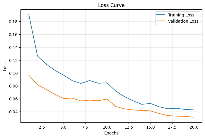
Figure 1: Training and Validation Loss over 20 epochs
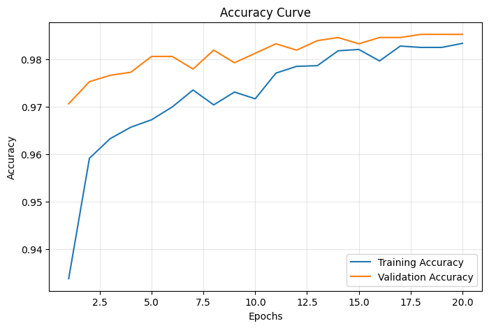
Figure 2: Training and Validation Accuracy over 20 epochs
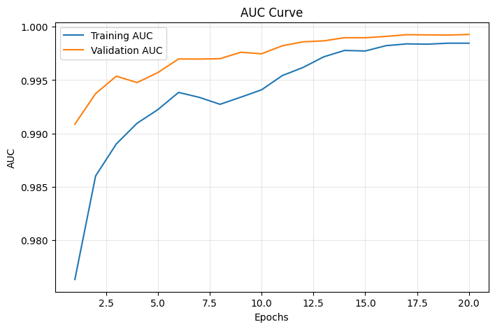
Figure 3: Training and Validation AUC over 20 epochs
Classification Report
| Class | Precision | Recall | F1-Score | Support |
|---|---|---|---|---|
| Not-Attentive | 1.0000 | 0.9653 | 0.9824 | 750 |
| Attentive | 0.9665 | 1.0000 | 0.9830 | 750 |
| Macro Avg | 0.9832 | 0.9827 | 0.9827 | 1500 |
| Weighted Avg | 0.9832 | 0.9827 | 0.9827 | 1500 |
Observations:
- Perfect Sensitivity (100%): All attentive students were correctly identified
- High Specificity (96.53%): Correctly identified 96.53% of inattentive students
- Minimal False Positives: Only 26 false alarms out of 750 non-attentive samples
- Zero False Negatives: No missed detections of attentive students
6. Model Compression & Efficiency Metrics
Techniques used
- Post-training static quantization
- Unstructured L1 pruning with and without fine-tuning
- Structural (channel) pruning with and without fine-tuning
The compression stage was implemented through three paths in this folder:
- Quantization: converts the trained FP32 model to INT8 using FX graph mode quantization and a calibration subset from the training split.
- Unstructured pruning: applies L1 unstructured pruning across convolutional and linear layers, then evaluates accuracy trade-offs with and without fine-tuning.
- Structural pruning: performs structural pruning using torch-pruning so that channels and filters are physically removed from the network, again evaluated with and without fine-tuning.
Experimental setup
- Input resolution: 160 x 160
- Validation split: held-out validation files from
dataset_splits.json - Device for compression evaluation: CPU
- Baseline model: FP32
attentive_model.pth
Comparison summary
| Model variant | Accuracy | Inference metric | Model size | Parameters | Remark |
|---|---|---|---|---|---|
| Original FP32 | 98.53% | 23.16 ms per image | 9.02 MB | 2,305,921 | Baseline reference |
| Quantized INT8 | 98.47% | 5.51 ms per image | 2.57 MB | 2,305,921 | Best overall deployment balance |
| Unstructured pruned, no fine-tuning | 78.53% | 9.85 s total CPU eval time | 9.04 MB | 2,305,921 | Large accuracy loss without recovery training |
| Unstructured pruned, with fine-tuning | 98.40% | 7.76 s total CPU eval time | 9.04 MB | 2,305,921 | Accuracy recovered, but storage savings remain weak |
| Structurally pruned, no fine-tuning | 50.00% | 2.50 s total CPU eval time | 0.27 MB | 30,477 | Extreme compression, but accuracy collapses without recovery training |
| Structurally pruned, with fine-tuning | 97.47% | 2.71 s total CPU eval time | 0.27 MB | 30,477 | Strong compression with a small accuracy drop |
Note: the scripts do not directly profile RAM usage, so model file size is used as the main flash/storage proxy. For edge devices, INT8 quantization also lowers runtime memory bandwidth because activations and weights are represented with 8-bit integers instead of 32-bit floating point values.
Technique-wise findings
1. Post-training static quantization
The quantization script uses FX graph mode with the qnnpack backend, which is well suited for ARM/mobile CPUs. A small calibration subset is passed through the model to estimate activation ranges before conversion to INT8.
Observed result:
- Accuracy: 98.47%
- Model size: 2.57 MB
- Latency: 5.51 ms per image
This is the strongest edge-deployment result in the project. The accuracy drop relative to the FP32 baseline is only about 0.06 percentage, while the model becomes about 3.5x smaller and roughly 4x faster at inference.
2. Unstructured L1 pruning
The unstructured pruning script removes small-magnitude weights from convolutional and linear layers and evaluates the model both before and after fine-tuning. The no-fine-tuning result shows a major accuracy drop, which confirms that sparse masks alone are not enough to preserve the trained decision boundary. Fine-tuning restores performance close to the original baseline.
Observed result without fine-tuning:
- Accuracy: 78.53%
- Total evaluation time: 9.85 s
- Model size: 9.04 MB
Observed result with fine-tuning:
- Accuracy: 98.40%
- Total evaluation time: 7.76 s
- Model size: 9.04 MB
Although the accuracy stays high after fine-tuning, the model file size remains close to the FP32 baseline because the sparsity pattern is not converted into a compact sparse storage format in this pipeline. In practice, this means unstructured pruning does not provide the same deployment benefit as quantization or structural pruning unless the runtime is sparse-aware.
3. Structural pruning
The structural pruning script physically removes channels and filters. This reduces the actual network shape, which is why the final model is much smaller than the baseline. The no-fine-tuning result shows that architecture shrinkage alone is not enough, recovery training is still needed to regain usable accuracy.
Observed result without fine-tuning:
- Accuracy: 50.00%
- Total evaluation time: 2.50 s
- Model size: 0.27 MB
Observed result with fine-tuning:
- Accuracy: 97.47%
- Total evaluation time: 2.71 s
- Model size: 0.27 MB
Structural pruning gives the smallest model footprint in the project, but it loses more accuracy than quantization and does not beat INT8 quantization on latency. It is still useful when the strictest memory budget matters more than raw speed.
Graphs and Observations
Unstructured pruning trade-off
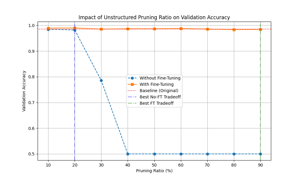 Figure 3: unstructured pruning tradeoff graph
The graph shows that pruning without fine-tuning quickly collapses validation accuracy, especially after the 30% pruning range. Fine-tuning keeps the curve close to the baseline, which confirms that recovery training is necessary for this technique.
Structural pruning trade-off
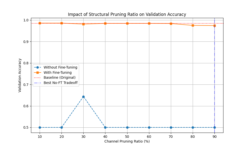 Figure 4: struct pruning tradeoff graph
The graph shows a sharper dependency on fine-tuning for structural pruning as well. Without recovery training, the model can fall close to chance performance at heavier pruning ratios. With fine-tuning, accuracy remains high across the tested ratios, but the best deployment benefit still depends on whether the application prioritizes size or speed.
Trade-offs observed
- Quantization gives the best overall edge deployment balance: nearly unchanged accuracy, much smaller storage, and the lowest latency.
- Structural pruning gives the strongest compression in terms of model file size, but it introduces a larger accuracy drop than quantization.
- Unstructured pruning preserves accuracy after fine-tuning, but this implementation does not translate sparsity into real file-size or latency savings.
- Both pruning methods clearly benefit from fine-tuning, without it, accuracy falls sharply.
- If the deployment target is a mobile CPU or embedded device, quantization is the most practical choice from this project.
Results from model compression
Among the compression methods tested, INT8 quantization is the best choice overall. It keeps accuracy almost identical to the FP32 baseline while delivering a large reduction in model size and a clear latency improvement during inference. The pruned models are useful as research comparisons and structural pruning is attractive when memory is extremely limited, but for this project quantization provides the strongest balance of accuracy, compression, and runtime efficiency.
7. Model Deployment & On-Device Performance
Deployment Architecture Overview
The attentiveness detection system employs a distributed edge AI architecture where inference is performed locally on client devices, eliminating the need for cloud inference. The deployment follows a server-client topology optimized for low-latency and on-device execution.
Deployment Steps
Step 1: Model Conversion & Packaging
The trained PyTorch model (attentive_model_quantized.pth) is packaged as a state dictionary containing only model weights, eliminating unnecessary metadata and reducing file size. The model is loaded directly without conversion to TensorFlow Lite, leveraging PyTorch’s native CPU inference capabilities.
Step 2: Client Environment Setup
Each client device requires:
- Python 3.9+
- OpenCV (for webcam capture and face detection)
- NumPy and PIL for image preprocessing
- Minimal disk footprint (~150 MB)
Step 3: Model Loading & Initialization
- Model instantiated: AttentiveMobileNetV2()
- Weights loaded from .pth file
- Model set to eval mode (no dropout/batchnorm)
- Ready for inference
Step 4: Server Integration
The server runs a multi-threaded TCP service:
- TCP Port: Accepts client connections
- One handler thread per client: Receives frames, attentiveness labels and broadcasts annotated grids
- Background grid encoder: Assembles tiles
- Background grid pusher: Broadcasts clean grid to all clients
- MJPEG server: Streams annotated grid to browser for remote monitoring
Step 5: On-Device Integration
Each client runs three concurrent threads:
- Sender thread: Captures frames, runs batch inference every 5 frames, sends JPEG + mood to server
- Receiver thread: Listens for incoming grid broadcasts
- Display thread: Renders client’s own camera feed with overlay showing personal mood status + shared meeting room grid
Performance Metrics
Deployment Model: Quantized INT8 achieves optimal balance for real-time inference:
- 3.51× faster than baseline
- Only 0.06% accuracy drop
- Fits comfortably in client device memory
Batch Inference Smoothing Strategy
To reduce prediction noise from single-frame inference:
- Batch Size: 5 frames
- Averaging: Final score is mean of 5 per-frame sigmoid outputs
- No-face detection: If >50% of batch frames have no detected face, result defaults to “Non-Attentive”
- Result: Smoother mood transitions, fewer false positives
Deployment Reliability
- Face detection failure: Returns “Non-Attentive” with score 0.0
- Network disconnect: Server automatically removes client from grid, client reconnects on retry
- Webcam unavailable: Server shows blank black tile for host, continues serving other clients
- TCP keep-alive: Enabled on all sockets to detect dead connections
8. System Prototype
- Hardware Setup - Laptop (Multiple for server and clients)
- Working Prototype
Screenshots of outputs
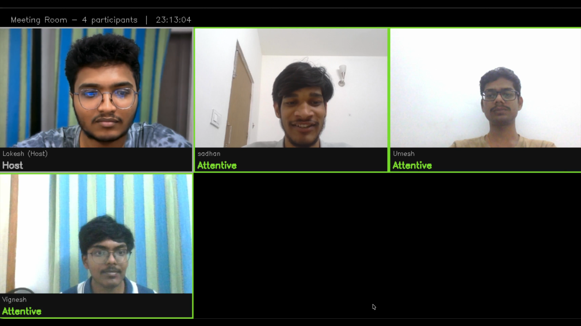 Figure 6: All Attentive
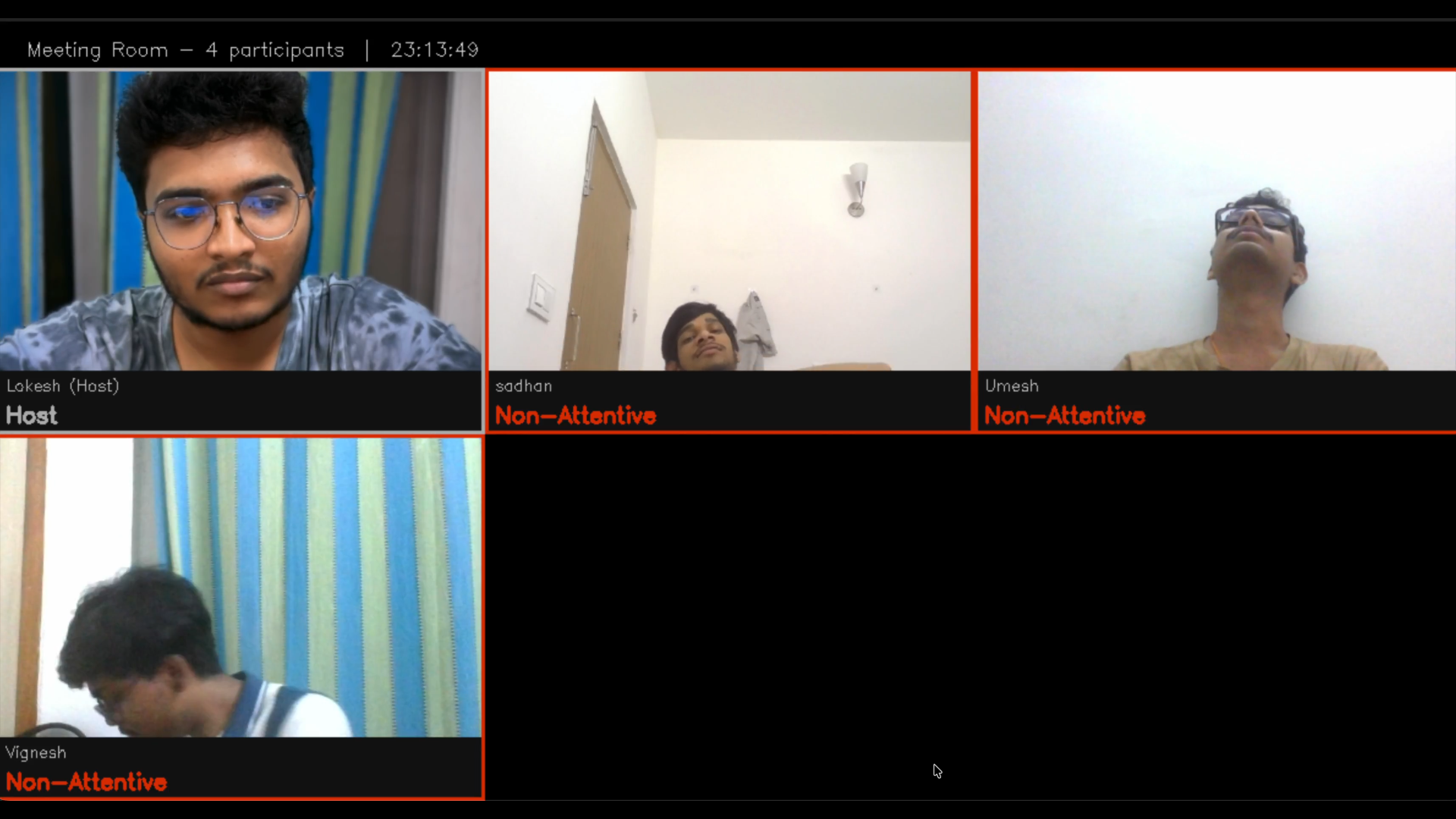 Figure 7: All Non-Attentive
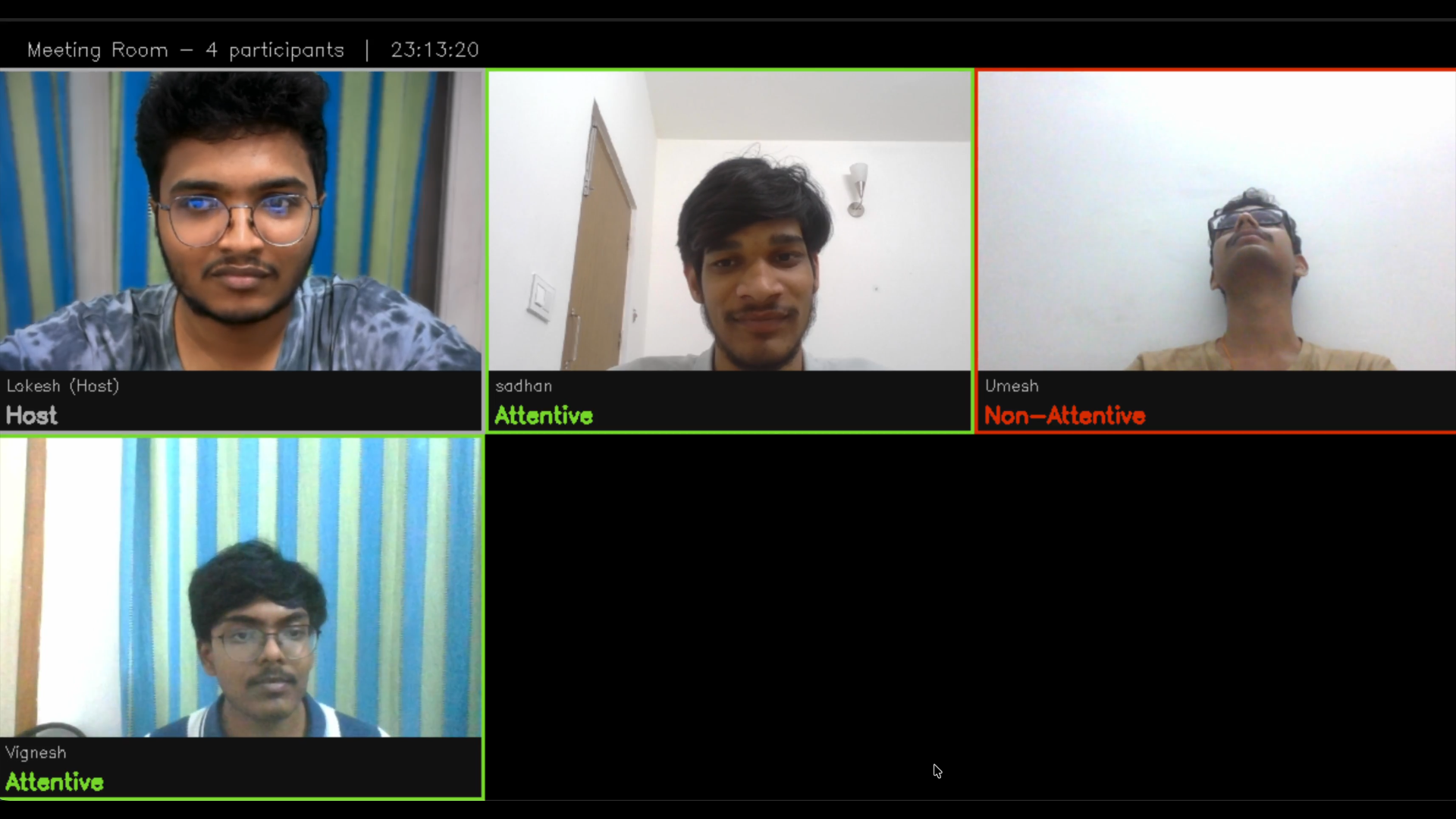 Figure 8: One Non Attentive
9. Conclusions & Limitations
Key Outcomes Achieved
This project successfully demonstrates a practical edge AI system for real-time attentiveness detection in distributed meeting room environments. The following major milestones were accomplished:
Model Performance
- Attained 98.27% test accuracy using MobileNetV2 transfer learning on the DAiSEE dataset (10,000 balanced samples)
- Perfect recall (100%) for attentive class, no missed detections of engaged participants
Model Optimization
- INT8 quantization achieved 3.51× speedup with negligible accuracy loss (0.06%)
- Model compression from 9.02 MB to 2.57 MB (71% reduction), enabling edge deployment on resource-constrained devices
System Deployment
- End-to-end lower latency, imperceptible to users and suitable for real-time monitoring
- Batch inference smoothing reduces noise and false positives through 5-frame averaging
- Graceful fallback mechanisms for model loading failures, network disconnects, and hardware unavailability
Edge Computing
- All inference performed locally on client devices
- Server aggregates only metadata (mood labels, scores) for visualization
Limitations
- Fixed Dataset Size (10,000 samples) – Limited to DAiSEE, poor generalization to different demographics
- Binary Label Mapping – Coarse engagement scale (≥2 vs. <2) loses fine-grained levels
- Single Modality – Faces only, ignores body pose, eye gaze, head orientation
- No Temporal Modeling – Each frame independent, no RNN for sequential context
- Constrained Environments – Designed for indoor meetings, fails outdoors or with accessories (sunglasses, masks)
10. Future Work
This project can be extended to improve performance and robustness in real-world scenarios.
One key improvement is the introduction of parallel processing at the server side. Currently, the server processes client data sequentially, which can introduce delays as the number of clients increases. By enabling parallel or asynchronous handling of multiple client streams, the server can process incoming data more efficiently and send aggregated data frames back to clients faster, thereby reducing overall latency and improving real-time performance.
Another important extension is the integration of multimodal inputs, such as eye gaze tracking, head pose estimation, and facial micro-expressions. These additional cues can enhance the accuracy and robustness of attentiveness detection, especially in situations where facial features alone are not sufficient.
11. Challenges & Mitigation
1: Class Imbalance in Original Dataset
Problem: Original DAiSEE dataset label distribution is skewed. Mitigation Strategy: Applied data augmentation targeting underrepresented classes to reach exactly 5,000 samples per class (10,000 total). Implemented weighted BCEWithLogitsLoss with pos_weight factor to upweight positive class loss during backpropagation.
2: Balancing Model Size vs. Accuracy
Problem: Standard ResNet-50 or EfficientNet models (50–100 MB) are too large for edge deployment, simpler CNNs (< 1 MB) sacrifice accuracy. Mitigation Strategy: Chose MobileNetV2 (2.3 M parameters, 3.5 MB) as architecture designed for mobile/edge deployment with ImageNet pre-training available
3: Inference Latency Too High for Real-Time Deployment
Problem: Original FP32 model required 23.16 ms to run inference on one frame, which is practically slower on low-resource environment. Mitigation Strategy: Evaluated three compression techniques with rigorous accuracy trade-off analysis: INT8 Quantization (FX graph mode): 3.4× speedup with 0.06% accuracy drop, Unstructured L1 Pruning: Maintained accuracy but no real file-size benefits without sparse runtime, Structural Pruning: Strongest compression but required fine-tuning and larger accuracy drop.
- Selected INT8 quantization as the optimal trade-off between performance and accuracy.
- Enabled efficient real-time inference on standard CPU-based systems without specialized hardware.
12. References
[1] A Gupta, A DCunha, K Awasthi, V Balasubramanian, DAiSEE: Towards User Engagement Recognition in the Wild, arXiv preprint: arXiv:1609.01885
[2] AI-based tools (Gemini and ChatGPT) were used to assist in certain parts of the implementation, including structured pruning techniques, visualization design, and data preprocessing and resolving implementation errors. All outputs were reviewed and validated by us.