🤖 Real-Time 2D Semantic Mapping
Instructor: Dr. Pandarasamy Arjunan
Team: Karney Jayanath, Shreevathsa K S, Rajneesh Babu
🌐 View Project Page →
A real-time, on-device semantic navigation aid for the visually impaired using Raspberry Pi 5 + Hailo-8 AI HAT (13 TOPS NPU). A pruned, INT8-quantized YOLOv8n model detects 20 indoor-relevant object classes at 24.7 FPS and fuses detections with gyroscope yaw from an Arduino Nicla Vision to build a live 2D polar semantic map — fully offline, no cloud, no GPU required.
Highlights
- True edge deployment — everything runs on RPi5 + Hailo-8; no cloud, no GPU, no internet required at runtime
- 5-stage compression pipeline — FP32 → PTQ → QAT → L1 Structured Pruning → Hailo HEF; pruned model achieves +9.4% mAP50 over the FP32 baseline
- 1.87× faster inference after pruning, at only 4.5 MB model size (HEF)
- Sensor fusion — IMU yaw from Nicla Vision combined with bounding-box geometry to compute real-world object heading and distance every frame
- Live dual-window display — Window 1: detection feed with labeled bounding boxes; Window 2: top-down 2D polar map with range rings at 1 m intervals
Repository Structure
.
├── Arduino Nicla Vision IMU/
│   ├── main_Nicla.py           # MicroPython IMU firmware for Arduino Nicla Vision (OpenMV IDE)
│   └── README.md               # Step 1: Nicla Vision setup guide
│
├── Colab Development flow/
│   ├── EDGE_SLAM.ipynb         # Full training + optimization + HEF compilation notebook
│   ├── README.md               # Steps 2 & 3: Colab training, ONNX export & HEF compilation
│   └── models/
│       ├── yolov8n_pruned.hef  # ✅ Compiled Hailo model — deploy this on RPi5 (4.3 MB)
│       ├── best_opset11.onnx   # Pruned YOLOv8n ONNX export, opset-11 (13 MB)
│       ├── yolov8n_pruned.har  # Hailo Archive — INT8-quantized intermediate (13 MB)
│       └── best_pruned.pt      # Pruned PyTorch checkpoint (6.3 MB)
│
├── RPI-Rpi5 deployment/
│   ├── main_RPI.py             # Edge runtime: Hailo inference + DFL decode + 2D semantic map
│   └── README.md               # Steps 4, 5 & 6: RPi5 setup, file transfer & run
│
├── report/
│   ├── edge_slam_report.pdf    # Full IEEE-format project report (LaTeX)
│   ├── edge_slam_report.tex    # LaTeX source
│   └── report_images/          # Benchmark charts and demo screenshots
│       ├── comparison_chart.png
│       ├── demo_detection_fps.jpg
│       ├── demo_detection_live.jpg
│       └── demo_semantic_map.jpg
│
└── README.md                   # Project overview + full report (this file)
Quick Navigation
| Folder | What’s inside | Guide |
|---|---|---|
Colab Development flow/ |
Training notebook + all compiled model files | Steps 2 & 3 → |
Colab Development flow/models/ |
yolov8n_pruned.hef, .onnx, .har, .pt |
Direct folder |
Arduino Nicla Vision IMU/ |
IMU firmware for Nicla Vision | Step 1 → |
RPI-Rpi5 deployment/ |
Edge inference script | Steps 4, 5 & 6 → |
report/ |
IEEE-format PDF report | PDF → |
Problem Statement
Visually impaired individuals navigate indoor environments with limited situational awareness. Existing assistive technologies — white canes, GPS-based devices — either lack real-time object-level perception or require connectivity. Recent edge AI hardware now makes it possible to run deep-learning perception pipelines on compact, battery-powered computers at interactive frame rates, at a fraction of the cost of specialized robotic platforms.
The challenge is threefold:
- Model compression: shrinking a capable detector to fit within the tight memory and compute budget of a consumer NPU
- NPU deployment: handling the non-standard multi-head output of YOLOv8 on a proprietary accelerator (Hailo-8) that requires its own compilation toolchain
- Sensor fusion: combining per-frame camera detections with continuous IMU yaw to maintain a persistent spatial model of nearby objects
Project Objectives
- Train and compress a YOLOv8n model for 20 indoor-relevant COCO classes using a reproducible Colab pipeline
- Compile the model to Hailo Executable Format (HEF) using the Hailo Dataflow Compiler (DFC)
- Deploy on Raspberry Pi 5 + Hailo-8 AI HAT at real-time frame rates
- Fuse detections with gyroscope yaw from a Nicla Vision IMU to estimate each object’s world heading and distance
- Display results as a live detection feed and a 2D top-down polar semantic map
Hardware & Software
Hardware
| Component | Model | Role |
|---|---|---|
| Main compute | Raspberry Pi 5 (8 GB) | Pre/post-processing, display |
| AI accelerator | Hailo-8 AI HAT | YOLOv8n HEF inference (13 TOPS, M.2 PCIe) |
| Camera | TNBA1392 (CSI ribbon) | RGB frame capture 640×480 |
| IMU sensor | Arduino Nicla Vision | Gyroscope yaw over USB serial (LSM6DSOX) |
| Power | USB-C power bank | Portable operation |
Physical connections:
TNBA1392 Camera  ── CSI ribbon ──► RPi5 CAM0
Hailo-8 AI HAT   ── M.2 / PCIe ──► RPi5 (stacked on top)
Nicla Vision     ── micro-USB  ──► RPi5 USB port
Power Bank       ── USB-C      ──► RPi5
Software
| Tool | Purpose |
|---|---|
| Google Colab (T4 GPU) | Model training and optimization |
| Ultralytics YOLOv8 | Base model and training framework |
| Hailo Dataflow Compiler v3.33.1 | ONNX → HEF compilation |
| HailoRT | On-device NPU inference |
| OpenMV IDE | Nicla Vision MicroPython firmware |
| Picamera2 | Camera capture on RPi5 |
| OpenCV | Frame display, drawing, NMS |
| pyserial | USB serial from Nicla IMU |
| pyttsx3 | Text-to-speech audio announcements |
| NumPy | DFL post-processing math |
Dataset
We used COCO128 (a 128-image subset of MS-COCO) for training, fine-tuning, and INT8 calibration. Only the 20 VI-relevant classes out of COCO’s 80 were used; all others were discarded.
Selected classes (COCO IDs):
| person (0) | backpack (24) | handbag (26) | suitcase (28) | bottle (39) | cup (41) |
|---|---|---|---|---|---|
| fork (42) | knife (43) | spoon (44) | bowl (45) | chair (56) | couch (57) |
| bed (59) | dining table (60) | laptop (63) | mouse (64) | remote (65) | keyboard (66) |
| cell phone (67) | book (73) |
Why these classes? Objects likely encountered in indoor home and office environments — furniture, tableware, personal items, and electronics — were retained. Outdoor and non-navigational classes (vehicles, animals, sports equipment) were excluded.
Dataset link: COCO128 on Ultralytics HUB — auto-downloaded when running the notebook.
Model: YOLOv8n
We start from the publicly pretrained YOLOv8n (nano) checkpoint and fine-tune it on our 20-class subset. YOLOv8 uses an anchor-free Detect head with Distribution Focal Loss (DFL) for bounding-box regression — which requires special handling on the Hailo NPU (see Deployment).
Architecture overview:
- Backbone: YOLOv8n CSPDarknet (lightweight)
- Neck: PANet feature pyramid
- Head: Anchor-free Detect → 3 scales (strides 8, 16, 32) → 6 raw output tensors
Why YOLOv8n? Smallest YOLO variant, designed for edge deployment. Its DFL head is more accurate than anchor-based heads at small model sizes.
Training & Optimization Pipeline
All training runs on Google Colab T4 GPU. The full notebook is in Colab Development flow/EDGE_SLAM.ipynb. The pipeline has 5 stages:
Stage 1 — FP32 Baseline Fine-Tuning
Fine-tune pretrained YOLOv8n for 20 epochs on COCO128, restricted to 20 target classes.
model = YOLO('yolov8n.pt')
model.train(data='coco128.yaml', epochs=20, imgsz=640,
            batch=16, device=0, classes=TARGET_CLASS_IDS)
| Result: mAP50 = 0.6269 | latency = 8.30 ms | size = 6.23 MB |
Stage 2 — Post-Training Quantization (PTQ, TensorRT INT8)
Converts FP32 weights to INT8 using 64 COCO128 calibration images — no retraining.
| Result: mAP50 = 0.6093 (−2.8%) | latency = 4.66 ms | 1.78× faster |
Stage 3 — Quantization-Aware Training (QAT)
Retrains with simulated INT8 quantization noise injected during forward pass for 20 epochs.
Result: mAP50 = 0.5944 (−5.2%) — COCO128 is too small for QAT to be effective; full COCO would be needed.
Stage 4 — L1 Structured Pruning + Fine-Tuning (Deployed)
Removes 20% of Conv2d filters ranked lowest by L1-norm. Unlike unstructured sparsity, filter removal produces a genuinely smaller dense model. Fine-tuned for 20 more epochs after pruning.
for name, module in model.named_modules():
    if isinstance(module, torch.nn.Conv2d):
        prune.l1_unstructured(module, name='weight', amount=0.2)
        prune.remove(module, 'weight')
| Result: mAP50 = 0.6793 (+8.4% over PTQ, +5.24% over baseline) | latency = 4.58 ms |
Removing noisy low-magnitude filters before quantization acts as implicit regularization — this is why pruning improves mAP rather than hurting it.
Stage 5 — Knowledge Distillation (Ablation Only)
YOLOv8s teacher generates pseudo-labels; pruned YOLOv8n student trains on them. Not deployed.
Result: mAP50 = 0.5904 (−4.86%) — KD needs the full COCO dataset to be effective.
Pipeline Summary
| Stage | mAP50 | FPS (T4) | Latency (ms) | Size (MB) |
|---|---|---|---|---|
| Baseline FP32 | 0.6269 | 120.5 | 8.30 | 6.23 |
| PTQ INT8 | 0.6093 | 214.4 | 4.66 | 5.57 |
| QAT INT8 | 0.5944 | 186.6 | 5.36 | 5.65 |
| Pruned INT8 (deployed) | 0.6793 | 218.3 | 4.58 | 5.65 |
| KD INT8 (ablation) | 0.5904 | 120.5 | 8.30 | 6.23 |
| Hailo HEF on RPi5 | — | 24.7 | 40.5 | 4.50 |
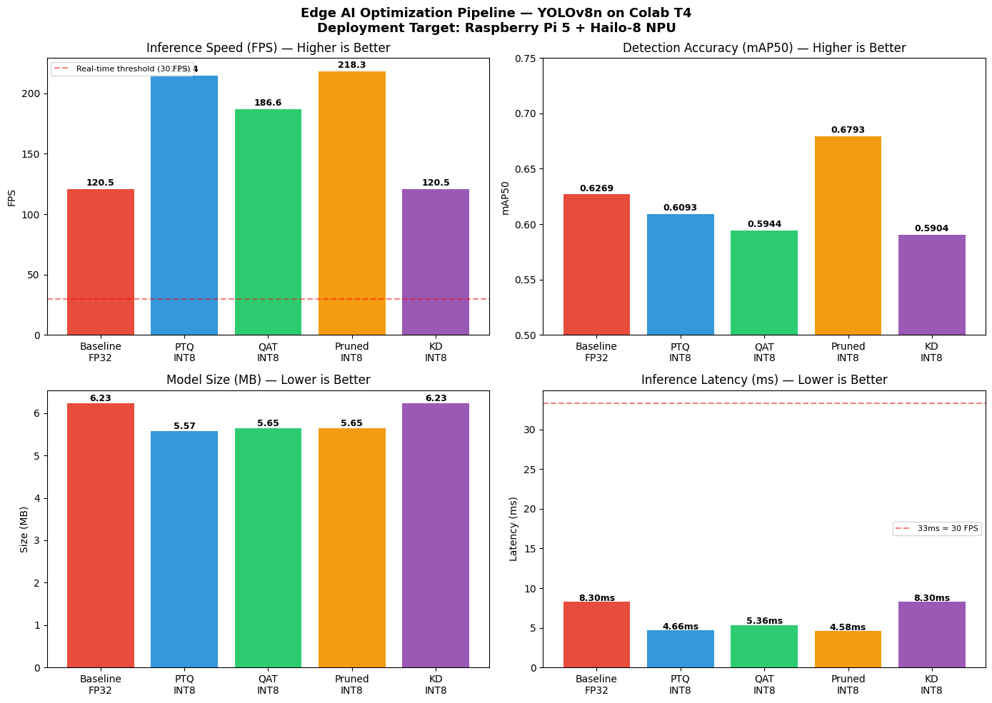
Figure 1: Four-panel benchmark chart (FPS, mAP50, model size, latency) across all optimization stages — from the Colab notebook output.
Deployment on RPi5 + Hailo-8
Hailo HEF Compilation (Colab Phase B)
The pruned model is exported to ONNX opset-11 (opset-13 uses operators unsupported by DFC) and compiled via:
ONNX (opset-11) → HAR → HAR (INT8 calibrated) → HEF (4.5 MB)
Note: HEF compilation requires Python 3.10 + Hailo DFC wheel (~488 MB, must be downloaded from hailo.ai). It is run in a separate Colab session after restarting the runtime. See
Colab Development flow/README.mdfor the full walkthrough.
DFL Decoding on RPi5 CPU
Hailo exports 6 raw tensors (3 box + 3 class). DFL decoding runs on the RPi5 CPU after every inference call:
# For each of 3 feature-map scales (stride s ∈ {8, 16, 32})
box_dist = (softmax(box_raw.reshape(H,W,4,16), axis=-1) * bins).sum(-1)
x1 = (cx + 0.5)*s - box_dist[...,0]*s
x2 = (cx + 0.5)*s + box_dist[...,2]*s
scores = sigmoid(cls_raw)
# → class-wise NMS (conf > 0.40, IoU < 0.45)
Nicla Vision IMU Streaming
Nicla Vision (MicroPython, OpenMV IDE) calibrates gyro bias over 300 samples (~3 s), applies a dead-band filter (±0.8°/s), and streams yaw angle continuously:
A:156.68 ← format: A:<angle_degrees>
The RPi5 reads from /dev/ttyACM0 in a background thread.
2D Semantic Map
Each detected object is placed on a polar map using:
- Camera FOV angle:
α_offset = ((cx − W/2) / (W/2)) × 30° - Absolute heading:
α_abs = (ψ_IMU + α_offset) mod 360° - Distance estimate:
d = max(0.3 m, h_ref / h_bbox)— reference height per class at 1 m - EMA smoothing (λ = 0.7) reduces per-frame jitter
Objects not seen for > 10 s are pruned. The 520×520 px OpenCV canvas shows range rings at 1 m intervals; dots are orange (< 2.5 m) or green (≥ 2.5 m).
Demo
Two OpenCV windows run simultaneously on the RPi5:
| Detection Feed | 2D Semantic Map |
|---|---|
 |
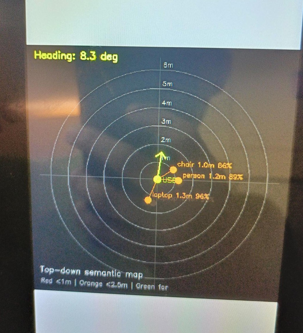 |
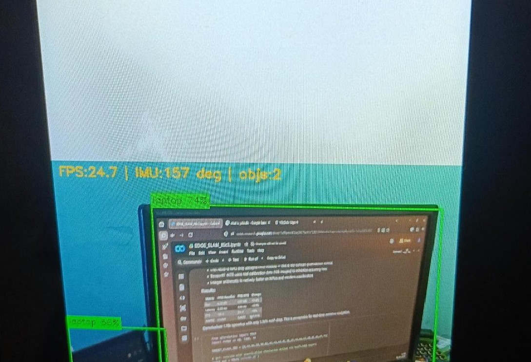
| Fig. 2: Laptop detected at 24.7 FPS, IMU heading 157° | Fig. 3: Chair 1.0 m (86%), person 1.2 m (89%), laptop 1.3 m (96%) |
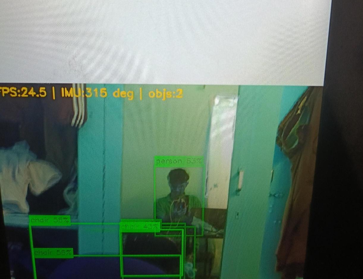
Fig. 4: Person (63%) and three chair instances (56%, 56%, 43%) detected simultaneously at 24.5 FPS, IMU heading 315°.
On-device performance:
| Metric | Value |
|---|---|
| Inference FPS (RPi5 + Hailo-8) | 24.7 FPS |
| HEF model size | 4.5 MB |
| Hailo clusters utilized | 8 / 8 |
| mAP50 gain vs FP32 | +9.4% |
| Speed-up vs FP32 | 1.87× |
| IMU yaw update rate | 50 Hz |
Step-by-Step Reproduction Guide
Step 1 — Nicla Vision Setup
Full guide:
Arduino Nicla Vision IMU/README.md
- Install OpenMV IDE from openmv.io
- Connect Nicla Vision to laptop via micro-USB → copy
Arduino Nicla Vision IMU/main_Nicla.pyto its internal disk → rename tomain.py - Open in OpenMV IDE → Connect → Run → verify
A:<angle>lines appear in serial monitor - Disconnect from laptop → plug into RPi5 USB port
- Hold the RPi5 still and vertical for 3 seconds after power-on (gyro bias calibration)
Step 2 — Colab Phase A (Training & ONNX Export)
Full guide:
Colab Development flow/README.md
- Open
Colab Development flow/EDGE_SLAM.ipynbin Google Colab (T4 GPU runtime) - Mount Google Drive — outputs save to
My Drive/edge_ai_project/ - Run all cells EXCEPT the last cell
- Covers: baseline → PTQ → QAT → L1 pruning → KD ablation → ONNX export
- The pruned ONNX model (
best_opset11.onnx) is saved to Google Drive
- Do NOT run the last cell yet
Step 3 — Colab Phase B (HEF Compilation)
Full guide:
Colab Development flow/README.md
The Hailo DFC requires Python 3.10 and is incompatible with Colab’s default environment and Blackwell CUDA libraries — a fresh session is mandatory.
- Go to hailo.ai → create a free account → log in
- Navigate: Downloads → AI Accelerator → AI Suite → Dataflow Compiler → Linux → x86 → Python 3.10
- Download
hailo_dataflow_compiler-3.33.1-py3-none-linux_x86_64.whl(~488 MB) - Upload the
.whltoMy Drive/edge_ai_project/ - Restart the Colab session → run only the last cell
- Grant Drive mount permission → the cell creates a Python 3.10 venv, installs DFC, and runs: Parse → Optimize (INT8, 64 calibration images, CPU-only) → Compile
- Download the output
yolov8n_pruned.hef(4.5 MB) to your laptop
Step 4 — RPi5 One-Time Setup
Full guide:
RPI-Rpi5 deployment/README.md
Connect via SSH (same Wi-Fi) or direct terminal:
# System packages
sudo apt install -y python3-venv python3-numpy python3-opencv \
  python3-serial python3-picamera2 v4l-utils rpicam-apps

# Hailo runtime
sudo apt install -y hailo-all

# Virtual environment
mkdir -p ~/edge_nav/models ~/edge_nav/logs
cd ~/edge_nav
python3 -m venv venv_edge_nav --system-site-packages
source ~/edge_nav/venv_edge_nav/bin/activate
pip install pyserial pyttsx3

# Verify
python -c "from hailo_platform import HEF, VDevice; print('Hailo OK')"
hailortcli fw-control identify
Step 5 — Transfer Files to RPi5
Full guide:
RPI-Rpi5 deployment/README.md
Run in Windows PowerShell (replace <RPI_IP> with the RPi5’s Wi-Fi IP):
scp "$env:USERPROFILE\Downloads\yolov8n_pruned.hef" `
    rpi15@<RPI_IP>:/home/rpi15/edge_nav/models/yolov8n_pruned.hef

scp "$env:USERPROFILE\Downloads\main_RPI.py" `
    rpi15@<RPI_IP>:/home/rpi15/edge_nav/main.py
Step 6 — Run the System
Full guide:
RPI-Rpi5 deployment/README.md
cd ~/edge_nav
source ~/edge_nav/venv_edge_nav/bin/activate
export DISPLAY=:0
python main.py
Two OpenCV windows open on the RPi5 display. Press q to quit.
Results & Analysis
Model Optimization Results
The L1-pruned INT8 model is the Pareto-optimal point across all metrics:
- mAP50 = 0.6793 — highest of all compression stages, +8.4% over PTQ and +5.24% over the FP32 baseline
- Latency = 4.58 ms on T4 GPU — 1.81× faster than FP32
- Size = 5.65 MB (ONNX) → 4.5 MB after Hailo HEF compilation
The pruning improvement is counterintuitive: removing 20% of filters with the lowest L1 norms eliminates the filters that contributed the most noise during quantization, giving the quantizer cleaner weight distributions to round. This acts as a form of quantization-friendly regularization.
On-Device Performance (RPi5 + Hailo-8)
| Metric | Value |
|---|---|
| Inference FPS | 24.7 FPS |
| HEF compilation time (Colab CPU) | ~8 minutes |
| Hailo-8 clusters used | 8 / 8 |
| Power draw (full system) | ~7–10 W (USB-C power bank) |
| IMU yaw latency | <20 ms (50 Hz polling) |
Limitations
- Distance estimation accuracy: The reference-height heuristic assumes objects are upright and at a fixed aspect ratio; cluttered scenes with partial occlusions reduce accuracy
- Gyro drift: Integrating yaw from a MEMS gyroscope introduces slow drift over long sessions (~1–2°/minute); a magnetometer or visual odometry would correct this
- COCO128 dataset: 128 images is too small for QAT and KD to generalize; these stages would outperform PTQ on the full 118K-image COCO dataset
- Indoor-only: The 20 selected classes are optimised for indoor navigation; outdoor deployment would require retraining
Planned Improvements
- Replace the reference-height distance heuristic with a lightweight monocular depth estimator (e.g., MiDaS-small) for more accurate distance
- Add visual odometry for drift-free position tracking over long sessions (the gyroscope-only yaw drifts gradually)
- Extend to a 3D voxel semantic map using depth + IMU fusion
- Detect more classes beyond the 20 currently used
- Port to a wearable form factor (e.g., glasses or vest-mounted)
- Run QAT and KD on the full COCO dataset for a fair comparison
Team
Course: CP330 — Edge AI, Department of Computational and Data Sciences, IISc Bengaluru
Instructor: Dr. Pandarasamy Arjunan
| Name | SR No. | Contribution |
|---|---|---|
| Karney Jayanath | 26831 | Model training & optimization — YOLOv8n fine-tuning, PTQ, QAT, L1 pruning, KD ablation, Colab pipeline, benchmarking |
| Shreevathsa K S | 25905 | RPi5 inference pipeline — Hailo HEF deployment, HailoRT integration, DFL decoder, Picamera2 capture loop, NMS, bounding-box rendering |
| Rajneesh Babu | 26058 | 2D semantic mapping — Nicla Vision IMU firmware, gyro calibration, yaw streaming, polar map, EMA smoothing, distance estimation |